Teaching Bioinformatics and Neuroinformatics by Using Free Web-based Tools
Abstract
This completely computer-based module's purpose is to introduce students to bioinformatics resources. We present an easy-to-adopt module that weaves together several important bioinformatic tools so students can grasp how these tools are used in answering research questions. Students integrate information gathered from websites dealing with anatomy (Mouse Brain Library), quantitative trait locus analysis (WebQTL from GeneNetwork), bioinformatics and gene expression analyses (University of California, Santa Cruz Genome Browser, National Center for Biotechnology Information's Entrez Gene, and the Allen Brain Atlas), and information resources (PubMed). Instructors can use these various websites in concert to teach genetics from the phenotypic level to the molecular level, aspects of neuroanatomy and histology, statistics, quantitative trait locus analysis, and molecular biology (including in situ hybridization and microarray analysis), and to introduce bioinformatic resources. Students use these resources to discover 1) the region(s) of chromosome(s) influencing the phenotypic trait, 2) a list of candidate genes—narrowed by expression data, 3) the in situ pattern of a given gene in the region of interest, 4) the nucleotide sequence of the candidate gene, and 5) articles describing the gene. Teaching materials such as a detailed student/instructor's manual, PowerPoints, sample exams, and links to free Web resources can be found at http://mdcune.psych.ucla.edu/modules/bioinformatics.
INTRODUCTION
Gregor Mendel's work was nearly lost (Maloney, 1996) and was only rediscovered well after his death in 1884. People with vision have created bioinformatic tools to prevent such a tragedy in our day. Students need experience with these tools to be well-trained scientists and even consumers of data; yet, undergraduate students are afforded little opportunity to learn about these resources that could become important tools in their careers. This article describes an easy-to-adopt module that weaves together several important bioinformatic tools so students can grasp the depth and power that these tools provide in formulating and answering research questions. Moreover, all of the resources used in this module are available for free on the Internet.
The core of this module is a quantitative trait locus (QTL) analysis, which has become an exciting topic in biology because it provides a means of linking variations in a quantitative phenotype to chromosomal loci. Furthermore, because the genotypes of so many organisms have been sequenced and published, QTL analyses can suggest candidate genes that could be involved in shaping the phenotype. QTL analyses are currently being applied to humans, animals, and even plants to determine the locus of genetically determined or influenced morphological and behavioral traits. Among the growing list of traits are olfactory bulb size (Williams et al., 2001), cerebellum size (Airey et al., 2002), cortex size (Beatty and Laughlin, 2006), alcoholism (Grisel, 2000; Bergen et al., 2003), Alzheimer's disease proteins (Ryman et al., 2008), attention-deficit hyperactivity disorder (Doyle et al., 2008), pain susceptibility (Nissenbaum et al., 2008), IQ (Butcher et al., 2008), obesity (Casellas et al., 2009), and dyslexia (Deffenbacher et al., 2004). In short, almost any morphological, physiological, or behavioral trait that could have at least some genetic basis can be examined by QTL analysis.
Besides experience with QTL analysis, this module also provides students with an integrated experience that goes from measuring phenotype through identifying candidate genes that are expressed in the tissue and that may influence the phenotype. As students journey through this module, they use a succession of bioinformatic tools, including the Mouse Brain Library; WebQTL from GeneNetwork; the University of California, Santa Cruz (UCSC) Genome Browser; National Center for Biotechnology Information (NCBI) Entrez Gene; the Allen Brain Atlas; and PubMed.
METHODS
Below, we provide a synopsis of the steps used in teaching this module. A more complete description is available in the student/instructor's manual and protocol PDFs that can be downloaded for free from our website at http://mdcune.psych.ucla.edu/modules/bioinformatics.
Quantifying the Phenotype
We use the Mouse Brain Library (Rosen et al., 2000; The Mouse Brain Library, 2005a,b) as a resource for our phenotype. This resource provides images of sectioned mouse brains from different recombinant inbred strains as well as pertinent metadata about individual animals, such as age, body weight, sex, and fresh brain weight. The set of images that we use come from brains that have been sectioned in the horizontal plane (Figure 1) and are Nissl stained, which defines cell bodies. The specific set of images that we use came from various BXD recombinant inbred strains (RISs) along with F0 C57BL/6 mice (B mice) and DBA/2J mice (D mice). Each BXD RIS has a unique recombination of the DNA from the F0 B and D mice on each chromosome. Good descriptions of the derivation of recombinant inbred strains can be found in Grisel (2000), Silver (2008), and at the GeneNetwork website (www.genenetwork.org). Also, each of these RISs have been genotyped, and informative markers have been mapped denoting whether the DNA was from the F0 B or D strain. Thus, RISs can be sorted as to whether they have the B or D marker at a given point on a given chromosome. Ultimately, differences in the phenotype among RISs can be correlated with differences in their genotypes. A good discussion of markers and chromosome mapping can be found in Silver's free online book on mouse genetics (Silver, 2008).
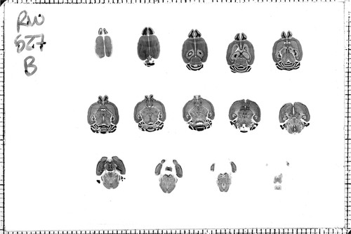
Figure 1. Image of a BXD mouse 527B from the Mouse Brain Library. This brain was sectioned in the horizontal plane at 30 μm, every 10th section was mounted and stained with cresyl violet for Nissl. Rostral is up.
Selection and Quantification of the Phenotype
Although any phenotypic brain trait could be selected, we selected the olfactory bulb for ease and reliability of quantification with less interobserver variability than other brain structures. Also, a published work on QTL analysis of mouse olfactory bulbs is available for comparison (Williams et al., 2001).
The specific set of images from the Mouse Brain Library that we use can be downloaded from our website at http://mdcune.psych.ucla.edu/modules/bioinformatics, along with a spreadsheet that contains the pertinent metadata (by kind permission of Dr. Robert W. Williams, Center for Genomics and Bioinformatics, University of Tennessee, purveyor of the Molecular Biology Laboratory).
To quantify the olfactory bulb as well as obtain an estimate of the volume of the whole brain, students download Image J (National Institutes of Health, 1997), a free software package that allows analyses of digital images. In brief, the entire olfactory bulb is traced in every section in which it occurs, and the volume is determined from these data.
Correcting Variability
QTL analyses are sensitive to various sources of variability—not just variability that is due to genotypic variation. Thus, a great deal of emphasis in this module is spent on controlling sources of variability that are not due to genotypic variation. Extraneous nongenotypic variability can come from technical or environmental sources (Williams, 1998) and will result in more type II statistical errors (false negatives) as long as it is not differentially distributed across strains. Some sources of variability that this module addresses are technical sources such as differential shrinkage of olfactory bulbs and interobserver variability, which we seek to minimize and correct (for details, see student/instructor's manual at http://mdcune.psych.ucla.edu/modules/bioinformatics).
Another important source of variability is inter-subject characteristics that could affect the phenotype apart from the genetic influences acting directly on our region of interest (olfactory bulbs). Brains from the Mouse Brain Library come from animals of diverse ages, body sizes, and brain weights as well as both sexes. To distill the variance uniquely due to genetic influences on olfactory bulbs, these extraneous variables must be controlled for statistically via multiple regression. This step provides an excellent opportunity to teach simple and multiple regression as tools for this purpose.
QTL Analysis by Using GeneNetwork
After removing extraneous variance, students then find an average of the residual variance for each recombinant inbred strain and are ready to perform the QTL analysis, by using WebQTL from GeneNetwork (Wang et al., 2003), a web-based resource provided by GeneNetwork From the University of Tennessee (2001). Again, QTL analysis relates the variation in the phenotype (or residual phenotype) to loci on chromosomes that impact the phenotype. See resources available at the GeneNetwork and Grisel (2000) for an excellent description of QTL analysis.
GeneNetwork uses a specific interface in which the data from a given trait can be entered, and a likelihood ratio statistic (LRS) is calculated as a function of markers across the genome (for a good discussion of the LRS, see Beatty and Laughlin, 2006). The LRS will be high if there is a large discrepancy in the phenotype between mice with the B versus D marker at a given chromosomal locus and low when the phenotypes are not discrepant. Large LRS values suggest that a gene(s) at or near the markers have a large impact on the phenotype (Figure 2).
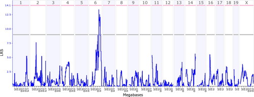
Figure 2. Output from WebQTL in GeneNetwork using students' data. This graph shows the likelihood ratio statistic (blue squiggly line) as a function of megabases across all mouse chromosomes except for Y. The criterion for significance is indicated by the pink horizontal line (genomewide p level—α level of 0.05), and the criterion for suggested is indicated by the gray horizontal line (genomewide p level of 0.67).
In our example (Figure 2), students can see that they obtained a peak LRS score on the distal end of chromosome 6 that exceeded the “suggested” criterion and approached the criterion for significance. Figure 3 shows the same graph as Figure 2 but “zoomed-in” on the peak so that only a part of chromosome 6 is displayed. On the top of the graph, there is a track linking directly to the UCSC Genome Browser.
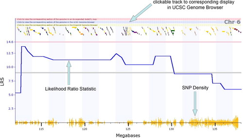
Figure 3. A “zoomed-in” section of chromosome 6 from the same data as displayed in Figure 2. This view shows the single nucleotide polymorphism (SNP) track as well as the LRS as a function of marker. Furthermore, there is a clickable track that leads directly to the UCSC Genome Browser for that particular portion of chromosome. The small colored boxes near the top of the figure represent individual genes and are also hot-linked to further information about individual genes.
Using the UCSC Genome Browser
The UCSC Genome Browser (Zweig et al., 2008, University of California Santa Cruz Genome Project, 2009) is a “site [that] contains the reference sequence and working draft assemblies for a large collection of genomes.” The UCSC Genome Browser provides a list of the known genes spatially arrayed in the selected region of a given chromosome. In Figure 4, the list of genes in the portion of chromosome 6 displayed in Figure 3 can be seen. Students then have a list of candidate genes that may influence the phenotype.
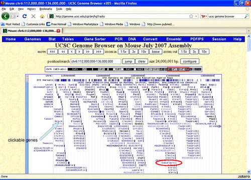
Figure 4. Screenshot of the UCSC Genome Browser for the span of chromosome 6 corresponding to the peak displayed in Figures 2 and 3. (The red box near top displays the portion of chromosome 6 displayed.) Here, we can see list of the known genes in this region of chromosome 6. Names are staggered with relation to where the gene would occur on the chromosome. These names are hot-linked to more information such as the relative degree of expression. As one example, the gene Gabarapl1 (γ-aminobutyric acid (A) receptor-associated protein-like 1) is a gene on the distal end of chromosome 6 and is known to be expressed in the olfactory bulb.
Students use the microarray data to refine the list of candidate genes. By clicking on the names of genes, students can link to the microarray data, which may include whether the gene is expressed in the olfactory bulb. These microarray data provide an opportunity to discuss this cutting-edge technique (Figure 5). As students identify genes that are expressed in the olfactory bulb, we have them pursue further information about these genes using other bioinformatic resources. The UCSC Genome Browser has links to several other bioinformatic resources such as the Allen Brain Atlas, NCBI Entrez Gene, and NCBI PubMed.
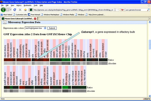
Figure 5. Screenshot from UCSC Genome Browser showing the expression of the Gabarapl1 gene in olfactory bulb relative to other tissues. Although the expression of Gabarapl1 is not extremely high, it might be of interest because it is a gene whose differential expression could affect development.
Using the Allen Brain Atlas
Once students have used the UCSC Genome Browser to identify a gene that is highly expressed in the olfactory bulb, they are then asked to click on the link to the Allen Brain Atlas (Lein et al., 2007; Allen Institute for Brain Science, 2009). The Allen Brain Atlas is an interactive, genome-wide image database of gene expression. In other words, it is a database of in situ hybridization studies showing the expression pattern of specific genes across brain regions (cf. Ramos et al., 2007). The Allen Brain Atlas gives students the opportunity to learn about in situ hybridization as well as some experience with a brain atlas and neuroanatomy.
Specifically, we ask students to describe which olfactory bulb cell layers express their particular gene of interest (Figure 6). Knowing which cell layers express the gene could give clues about the ontogeny of size differences among strains. Using the Allen Brain Atlas brings the students full circle back to the tissue itself, this time armed with the knowledge of a gene that could have affected the development of this structure.
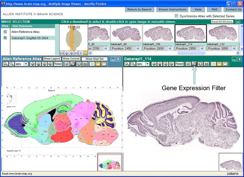
Figure 6. Screenshot from the Allen Brain Atlas. Large panel on right shows the in situ expression in a parasagittal section. Because Gabarapl1 is widely expressed, most of the brain shows some expression of this gene but highly expressed (darker) regions include the olfactory bulb, hippocampus, and one cortical layer. Large panel on the left is a plate from the corresponding atlas so that students can identify the names of the cell layers in which this gene is expressed.
Using Entrez Gene
Once genes expressed in the olfactory bulb have been identified, students can use a link from the UCSC Genome Browser to the NCBI Entrez Gene resource (NCBI, 2009a). Using a link out of the UCSC Genome Browser, we have students find the nucleotide sequence of the gene as well as the coding sequence (Figure 7). We use this as an opportunity to talk about introns and exons and why the whole nucleotide sequence does not always coincide to the coding sequence. Students learn that this information is useful for constructing in situ probes, quantitative polymerase chain reaction, or antibodies to study the expression of this gene during development.
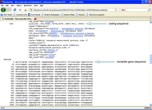
Figure 7. Screenshot from Entrez Gene displaying information about the coding sequence and the nucleotide sequence of the gene.
Using PubMed
When students locate a gene that is expressed in the olfactory bulb, we ask students to find an article about that particular gene and include a summary of the article in their write-up. The UCSC Genome Browser provides a direct link to a listing of the relevant articles in PubMed (NCBI, 2009b). Although some institutions may have limited library resources, many journals now have content online for free (listings can be found at the Open Directory Project, 2002), and PubMed Central provides articles for free. We ask students to find an article that describes something about their gene, preferably relating to function, and write an abstract of the article.
Implementing the Bioinformatics Module
Our module is laid out in 3 wk of lab instruction (3 h of lecture with three 3-h lab periods). We have a large number of students (40–150) in any given term, so we distribute the work accordingly and have students serve as “checks” on each other's accuracy by assigning more than one student the same set of mice. Instructors with small enrollments may need to adjust the workload per student or the number of weeks devoted to this module to quantify the phenotype in an adequate sample of mice (three to four) in each RIS.
Our students are either psychobiology or neuroscience juniors and seniors. All students have had a course in statistics, a course in genetics, and some exposure to neuroanatomy. Nonetheless, in teaching this module, we review relevant statistics, genetics, and neuroanatomy. Thus, prerequisite courses in statistics, neuroanatomy, or genetics are probably not necessary if the instructor provides relevant background on these topics.
Assessing the Effectiveness of This Module
To assess the effectiveness of this module, we administered a brief quiz to measure gains not only in the content of this module but also to tap understanding of statistics and logical reasoning before and after exposure to the module (a pre- and posttest design). (The quiz can be viewed in the Supplemental Material). In our analyses of the quiz data, we threw out question 11 due to poor psychometric properties and question 16 because of a wording error on the original item—now fixed. Nonetheless, even when these items were included the pattern of significant differences was maintained. Because repeated testing can sometimes raise scores by itself (Campbell and Stanley, 1963; Trochim, 1986, 2006), we controlled for this possibility by administering only the posttest in one of the two samples of students.
To assess student perspectives on their learning, we administered a satisfaction survey based on a series of questions with Likert-scaled response options. (Survey can be viewed in the Supplemental Material). Students were also asked to respond to the open-ended question, “Please describe the purpose of the QTL (Bioinformatics) module from a learning standpoint in the space below.” No further prompts were given and students were not limited on the length of their response. No specific responses were anticipated before data collection, so the coding of data was loosely based on a grounded theory model that allowed student perceptions to emerge without a preconceived hypothesis. Nonetheless, given the nature of the module, there was a strong likelihood that students would comment on content knowledge, the relevance of statistics, and the usefulness of the technology. All assessment measures had Institutional Review Board (IRB) approval (UCLA IRB Exemption 07-211).
The participants consisted of 92 volunteers from UCLA's fall 2008 Psychology 116, Psychobiology Lab (who received the pretest and posttest) and 39 volunteers from winter 2009 Neuroscience 101L, Neuroscience Lab (who only received the posttest). Both courses have students with very similar demographics and career ambitions. Responses to the Likert and qualitative items were pooled across both samples of students.
RESULTS
We have taught this module for several terms and invariably found evidence to support that it was an effective learning exercise. When comparing posttest to pretest scores using a paired t test, highly significant gains were found (t91 = 14.58, p < 0.001; Figure 8). Students who only took the posttest still showed gains relative to the previous term's pretest (t129 = 10.61, p < 0.001—independent t test). Posttest scores did not differ between students who had the pretest and those who did not (t129 = 0.06, p > 0.95—independent t test; Figure 8). The latter results establish that the gains that we observed are probably due to the instructional module and not due to a confounding factor such as “pretest sensitization” (Campbell and Stanley, 1963; Trochim, 1986, 2006). Pretest scores did not significantly correlate with grades on this unit (r84 = 0.164, p > 0.10), suggesting that differential student performance was not due to some students being better prepared than others but rather due to genuine gains in learning. Posttest scores did correlate with the grades on the unit (r84 = 0.537, p < 0.001) when grades were determined by a multiple-choice and a short-answer exam but not in the subsequent term when grades were only determined by a short-answer exam (r34 = 0.087, p > 0.60).
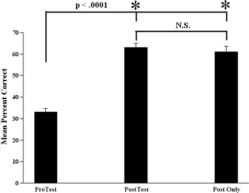
Figure 8. Mean (± standard error of mean) percentage correct on pretest and posttest given in one academic term and a posttest alone given in a subsequent term. Asterisks indicate significant differences as determined by a paired t test (for tests given in same term) and an independent t test for tests given in different terms. N.S., difference not significant.
On the satisfaction survey, students indicated that their understanding of bioinformatics databases was enhanced, as was their understanding of statistics, genetics, and molecular biology (Figure 9). (See Supplemental Material to view the survey and to see responses question by question.)
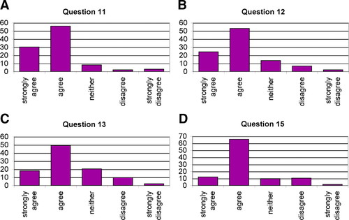
Figure 9. Percentage of respondents (n = 132) as a function of scale points. Questions were worded as follows. (A) Question 11: My understanding of bioinformatics databases was enhanced by actually doing the computer tasks and examining their data. (B) Question 12: My understanding of genetics was enhanced by the QTL (Bioinformatics) module. (C) Question 13: My understanding of statistics was enhanced by the QTL (Bioinformatics) module. (D) Question 15: I learned something about molecular biology from the QTL (Bioinformatics) module.
Most responses to the open-ended question, “Please describe the purpose of the QTL (Bioinformatics) module from a learning standpoint in the space below” described a combination of learning objectives that factored down to six main categories: 1) illustrative, 2) content knowledge, 3) hands-on learning, 4) technology, 5) statistics, and 6) job related. Responses coded as illustrative addressed the module's ability to disseminate knowledge without reference to applying skills or analyzing content (responses included terminology such as “exposed,” “showed,” “familiarize” or “to see how”). Responses were coded as content knowledge if the response acknowledged that learning the material was at least one objective for using the QTL module. Responses that addressed the module's ability to provide an experience to perform a learning-based task were coded as hands-on learning (responses included phrases such as “doing the activity,” “opportunity to participate,” “allows us to locate and analyze,” or “hands-on approach”). The technology category incorporated all responses that described learning objectives related to using bioinformatic tools, learning about a computer program or application, or developing computer-related skills. The statistics category included any responses that described the QTL module's usefulness for analyzing data. Finally, responses that claimed that learning to use the QTL module helped prepare students for “work in the field,” “real world experiments,” or “going into research” were categorized as job related. Table 1 shows the frequency of responses by category, along with cross-tab data on four categories that had a higher rate of correlation: hands-on learning and technology, and technology and job related. Frequency data are also provided on student satisfaction levels, even though the question did not require such commentary. Most student comments were not value based and simply stated the perceived purpose of the QTL module; however, several students offered their opinion of the module's usefulness. Twenty-seven comments included positive adjectives or phrases within the response, such as “reinforced learning,” “makes learning easier,” “quick and efficient,” or “greatly enhanced [learning].” Five comments included negative adjectives or phrases within the response, such as “too fast-paced,” “confusing,” or “busy work.”
| Category | Frequency |
|---|---|
| Purpose | |
| Illustrative | 67 |
| Content knowledge | 62 |
| Hands-on learning | 56 |
| Technology | 42 |
| Statistics | 26 |
| Job related | 26 |
| Frequently correlated categories | |
| Hands-on learning/technology | 23 |
| Technology/job related | 15 |
| Satisfaction | |
| Positive comments | 27 |
| Negative comments | 5 |
DISCUSSION
Both the content-based and attitudinal data indicate that this module is a successful pedagogical unit. The dramatic differences in the pretest versus the posttest results clearly show that students made gains in knowledge acquisition, as well as quantitative reasoning skills. The satisfaction survey reflected students' impression that their understanding of genetics, statistics, and molecular biology was enhanced by this module. In addition, student responses supported the module's ability to provide hands-on, learning-based tasks, which fostered their ability to master technology, statistics, and job- and career-related skills. Rightfully, no student mistook the module for a simulation when addressing its purpose in the open-ended question. Rather, students understood that they used these digital tools just as professional investigators would when conducting research. Finally, even though the open-ended question did not specifically solicit value judgments, students' positive comments outweighed negative comments by a ratio of 5:1.
With regard to the QTL data produced, our students almost invariably found a peak on the distal end of chromosome 6 that reached the “suggested” level, but not quite the significant level (Figure 2). We have replicated this finding across several terms using different sets of students, and this result is quite robust. Suggested peaks are worthy of further pursuit because 1) QTL analysis is a tool for generating a list of genes that might influence the phenotype and suggested peaks probably should not be ignored; 2) the α level for individual points is extremely stringent, so it is actually difficult to find a significant peak; and 3) student data probably underestimate the true relationship between markers and phenotype. When dealing with inexperienced students taking measurements, error variance will probably be large, thus diluting the relationship between markers and the phenotype. Furthermore, suggested relationships are reported in the literature (Beatty and Laughlin, 2006 ; Doyle et al., 2008; Ryman et al., 2008; but also see Williams, 1998). Therefore, instructors should feel gratified when their students can at least find peaks that reach the suggested criterion and use these peaks to generate a list of genes that have a putative impact on the phenotype.
Notably, our students did not faithfully replicate the findings of Williams et al. (2001). Instead, our students found fewer QTL peaks, and although our students did find a peak on chromosome 6, it was shifted relative to Williams et al. (2001). There are several possible reasons for these differences: 1) we used a slightly different set of strains—Williams et al. (2001) used F1 mice and we did not; 2) in contrast to Williams et al. (2001), we used volumes rather than weight; 3) for greater consistency among students, we operationally define the olfactory bulb in a slightly different manner than do Williams et al. (2001); 4) the map that we were using probably had more markers than Williams et al. (2001) had, so our peak may be more refined; and 5) the difference in the number of QTL peaks was probably due to our students' data having considerably more error variance than Williams et al. (2001). Accordingly, the probability of making a type II error (false negative) is higher with our student data, which would mean fewer peaks. We used this as a lesson on what random error variance does to data and why it pays to be painstaking in science.
We used the olfactory bulb in this module because inexperienced students could reliably quantify the phenotype and because there is a published work on this structure to which students can compare their data. Nonetheless, many other brain phenotypes could easily be substituted, such as cerebellum, hippocampus, corpus callosum, and cortex size. Published papers are available on each of these brain phenotypes (LeRoy et al., 1998; Airey et al., 2002; Peirce et al., 2003; Beatty and Laughlin, 2006).
This module not only exposes students to QTL analysis, which is a relatively new tool in molecular biology/genetics but also exposes them to various bioinformatic tools weaving them together into a cohesive, comprehensible unit. Giving students experience with these tools sharpens their understanding of the underlying biology and statistics that were used to construct these bioinformatic tools. Our ultimate goal goes beyond exposing students to these resources; it also includes guiding students in solving a tractable problem by using this module as a vehicle to teach statistical analyses, genetics, neuroanatomy, and molecular biology. Although we do not use all of the many features available at GeneNetwork, the UCSC Genome Browser (Zweig et al., 2008), the Allen Brain Atlas (cf. Ramos et al., 2007), and NCBI databases, we do manage to expose students to these enormously valuable tools that are being used daily in research. The fundamental analytical and research skills acquired in this module would be valuable and applicable to any student's future career.
From the instructor's point of view, this teaching module is easy to implement. In the course of teaching this unit, we identified and remedied many obstacles to make it a better learning experience for both students and instructors. Notably, we have vetted the set of images used from the Mouse Brain Library so that they are the most complete ones available for the RISs used. Also, we have discovered that even when students have a background in statistics and genetics, they still need a refresher tutorial. To assist faculty with these tutorials, we have provided PowerPoint tutorial slides that focus on statistics and other topics in this module on our website at http://mdcune.psych.ucla.edu/modules/bioinformatics (instructors must register as faculty for access to PowerPoints). Because this module is inquiry based, even though the outcome is fairly predictable, it does vary—usually depending on the care with which the students approach the material. Thus, it remains an interesting unit to teach across several terms. Finally, as the bioinformatic tools continue to improve, this module will provide for more opportunities to explore different phenotypes. Soon, high-resolution images ought to be available in the Mouse Brain Library, allowing cell-by-cell resolution that would open up a new realm to student exploration of the relationship of brain phenotypes to genotypes.
Notably, all of the web-based resources used in the module are available free to users. As a result, this module can be used by any faculty with access to computers. We have republished (with permission) the set of images from the Mouse Brain Library as well as a spreadsheet that contains the metadata about these mice to save instructors time in implementing this module. These and other didactic materials, such as a detailed student/instructor's manual, PDFs of handouts, PowerPoint slides, and sample exams, are available for free at our website at http://mdcune.psych.ucla.edu/modules/bioinformatics.
ACKNOWLEDGMENTS
We thank A.-M. Schaaf for help in preparing this manuscript and Rick Laughlin for help in instructing this module. This study was supported by National Science Foundation grant CCLI DUE-0717306 (to W. G.) and a grant from the UCLA Office of Instructional Development (to W. G.).


