Mathematical Manipulative Models: In Defense of “Beanbag Biology”
Abstract
Mathematical manipulative models have had a long history of influence in biological research and in secondary school education, but they are frequently neglected in undergraduate biology education. By linking mathematical manipulative models in a four-step process—1) use of physical manipulatives, 2) interactive exploration of computer simulations, 3) derivation of mathematical relationships from core principles, and 4) analysis of real data sets—we demonstrate a process that we have shared in biological faculty development workshops led by staff from the BioQUEST Curriculum Consortium over the past 24 yr. We built this approach based upon a broad survey of literature in mathematical educational research that has convincingly demonstrated the utility of multiple models that involve physical, kinesthetic learning to actual data and interactive simulations. Two projects that use this approach are introduced: The Biological Excel Simulations and Tools in Exploratory, Experiential Mathematics (ESTEEM) Project (http://bioquest.org/esteem) and Numerical Undergraduate Mathematical Biology Education (NUMB3R5 COUNT; http://bioquest.org/numberscount). Examples here emphasize genetics, ecology, population biology, photosynthesis, cancer, and epidemiology. Mathematical manipulative models help learners break through prior fears to develop an appreciation for how mathematical reasoning informs problem solving, inference, and precise communication in biology and enhance the diversity of quantitative biology education.
INTRODUCTION
Numerous national commissions have emphasized mathematical fluency as a crucial component of educational reform in biology. Nonetheless, biology curricula at most institutions remain resolutely free of meaningful quantitative reasoning and analysis. To break this impasse, we propose a pedagogical approach that approaches mathematics from four complementary perspectives: 1) physical manipulatives, 2) computer simulations, 3) derivation of mathematical relationships from core principles, and 4) analysis of real data sets. We demonstrate this approach with specific examples taken from the BioQUEST Curriculum Consortium's 24-yr experience of holding faculty development workshops for biology and mathematics educators. In these workshops, we have frequently found that manipulatives help learners break through prior fears to develop an appreciation for how mathematical reasoning informs problem solving, inference, and precise communication in biology.
Unfortunately, two main concerns have hindered the adoption of manipulatives in undergraduate science education. Some faculty worry that college students are already skilled in abstract thinking and will therefore view use of manipulatives as condescending. Furthermore, students' experience with sophisticated and interactive visualizations from computer gaming may make physical manipulatives seem hopelessly outdated. What, then, do manipulatives have to offer?
First, many studies provide evidence that appropriate classroom use of manipulatives both broadens and deepens students' learning of mathematical concepts. For example, group work with manipulatives transforms mathematical problem solving into a social activity, decreasing student anxiety and increasing engagement (Eyster and Tashiro, 1997; Sowey, 2001). Kinesthetic learners in particular benefit from the opportunity to apply abstract concepts to real-world examples. Similarly, working with manipulatives helps students develop problem-solving and critical-thinking skills (Eyster and Tashiro, 1997); increases students' sense of responsibility for their own learning; and emphasizes intuitive, long-term understanding of course material (Shaughnessy, 1992; Sowey, 2001; also see Jungck et al., 2000a,b). A meta-analysis of 60 research studies concluded that consistent and knowledgeable use of manipulatives improves both students' mathematical achievement and their attitudes toward mathematics (Sowell, 1989). Given this strong consensus, we focus here on the more conceptual aspects of using manipulative models.
Second, mathematical manipulatives play key roles in both the history and the contemporary practice of biology. Some of the most famous examples include Watson and Crick's model of the DNA double helix, Hodgkin's physical model of insulin's three-dimensional structure, Pauling's paper model of a protein α-helix, camera models of eyes, and Caspar's and Klug's polyhedral models of viral capsids. More recently, a 3.5-m-tall sculpture depicting the forces exerted by lung cells during angiogenesis tied for first place in Science magazine's 2009 International Science & Engineering Visualization Challenge. Classroom use of manipulatives helps demonstrate the importance of structural models in scientific discovery and communication.
Beanbag Biology: History of a Phrase
In a famous passage in his book Animal Species and Evolution, biologist Ernst Mayr (1963) criticized the mathematical basis of modern population genetics as mere “beanbag genetics” that ignored the complex patterns of interactions between genes. J.B.S. Haldane, one of the founders of population genetics, countered (1964) that mathematical analysis enables evolutionary biologists to make more precise and quantitative predictions, avoiding much of the clutter and vagueness of purely verbal arguments. This article was recently reprinted (Haldane, 2008), along with several articles that comment on Haldane's perspective. Although these papers deal with metaphorical beanbags, they lay a propitious foundation for considering the role of physical manipulatives—actual, physical beanbags—in biological classroom activities. In this essay, we explore the uses of true beanbag biology for student learning.
BEANBAG MATHEMATICAL BIOLOGY
Game 1: Outbreak in a Cup
Many mathematical models have been used to explore the dynamics and control of infectious diseases. The basic framework of these models is to divide the population into groups according to their disease status: susceptible to the disease, infected and infectious, recovered and immune, and so on. The model then estimates the movement of individuals between these disease groups. To demonstrate how to develop such a model and explore the dynamics of a disease in a population, we developed a simple hands-on exercise.
Game 1a. Students are divided into small groups of two to four students. Each group is given one empty cup (the “experiment” cup), a second cup containing approximately 50 brown beans (kidney beans work well and an inexpensive 1-lb bag is usually enough for a class of 24), and a third cup with approximately 50 white beans (navy or northern beans provided they are approximately the same shape as the kidney beans). Each group then sets up the initial scenario by placing 20 brown beans and one white bean into the experiment cup. The students are then instructed to repeat the following set of steps:
Without looking in the cup, a student from the group selects two beans from the cup.
If both beans are the same color, the student simply returns the beans.
If one bean is brown and the other white, the student removes the brown bean and returns two white beans to the cup.
At each time step, record the event that occurs: either no change or a new infection.
Repeat this process until told to stop.
This simple game demonstrates how a disease could move through a population. It is important to discuss the assumptions that underlie this model. For example, no one recovers from this disease. Discussions about these assumptions can lead to any number of variations on this game. For example, some variations could be as follows:
Reduction in spread rate. Provide the students with a coin to flip when they get the one brown, one white draw. Transmission (e.g., replacing the brown with a white) only occurs if they flip heads.
Vaccination. Using a third color of beans (e.g., beige garbanzo beans or green peas, again making sure there is no difference in size or shape), replace a certain number of susceptible (brown) beans with vaccinated (beige) beans. Track the differences in the number of new infections as a function of percentage of the population vaccinated.
Recovery. Similarly to the vaccination, use red beans to replace a random infected (white) bean after a given number of draws or at announced times.
Game 1b. Another model of such a susceptible–infectious–recovered (S-I-R) scenario that is more visual for some students is Joan Aron's Reed-Frost model (see Wahlström et al., 1998; Figure 1). In this case, four colors of marbles are used and are randomly distributed into a linear trough: the three classes S, I, and R and a fourth color marble that adjusts the probability of contact between elements in that group of three. For example, if students decide that for a susceptible individual to become infected it has to be adjacent to an infectious individual, the probability of this happening will be affected not only by the amounts of each of the three S-I-R classes but also by this barrier population. We have found this model particularly helpful because multiple groups playing at one time usually make up their rules (and hence their intuitive mathematical models) quite differently, and we can have excellent discussions about the plausibility of different assumptions based on whether the disease is like measles, smallpox, acquired immunodeficiency syndrome, flu, common cold, or polio.
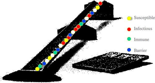
Figure 1. Reed–Frost epidemic SIR model. Mechanical model elaborated by Paul Fine with computer model by Dallas E. Wrege and Joan L. Aron, Johns Hopkins University (private communication). See Aron (2000).
After the students have built a physical model, we next have them analyze computational models of the same system. This activity can use either specialized epidemiological software such as SIR BuildIt (Weisstein and Gaff, unpublished data; Figure 2), Epidemiology (Udovic and Goodwin, 1998), and EcoBeaker (SimBiotic Software, 2010) or more general modeling software such as NetLogo (Wilensky, 1999), Mathematica, and Berkeley–Madonna. By adjusting individual model parameters, students can first develop and then test their intuitive understanding of the forces that determine an epidemic's progress through a population.
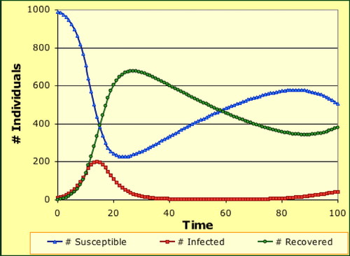
Figure 2. A spreadsheet SIR model of an epidemic (Weisstein and Gaff, unpublished data).
By now, students have played with a physical game, modified parameters in a computer model, and interpreted graphs showing the progress of specific diseases that differ in mode and ease of transmission, incubation period, and susceptibility to treatment. For a fourth and final perspective, students link their experience to the formal equations governing an SIR model (Jungck, 1997; Cohen, 2004). By relating these equations to the manipulatives and simulations they have already used, students can quickly grasp the equations' meaning, even if they have not had exposure to calculus per se (Figure 3).
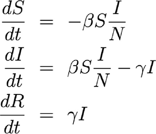
Figure 3. These three differential equations show the rate of change in the populations of susceptible individuals (dS/dt), infectious individuals (dI/dt), and recovered individuals (dR/dt). The parameter β measures the probability of disease transmission from an infectious to a susceptible individual, and γ is the recovery rate (see Gaff and Schaefer, 2009).
Once students have experience with the manipulatives, computer simulations, and equations, educators can use case studies to connect the course material to current and recent events. Many case studies exist on infectious diseases such as human immunodeficiency virus (HIV), West Nile virus, and H1N1 influenza (e.g., Waterman and Stanley, 2005).
Game 2: How Big Is this Population? Mark–Recapture Sampling Estimates
One of the biggest challenges in studying wild populations is to gauge the size of the population. A fairly simple technique that has been used for many years is a mark–recapture methodology. A sample of the population is trapped, and these individuals are marked in some noninvasive manner and released. A later sample then tracks how many individuals of the new sample were caught and marked in the previous sample. To improve students' intuitive understanding of this method and its limitations, we have developed another hands-on bead experiment.
Once again, we divide students into groups of two to four, and we provide them with two cups containing beans or beads of contrasting colors and an empty cup to hold the extra beads. The cups should be large enough such that the students can get a hand into the cup but not so large that they can select more than a small number of the beads. The students are instructed to repeat the following experiment:
Select a handful of beads from the cup of blue beads.
Count the blue beads and put them in the empty cup. Record this number.
Add one white bead for each blue bead taken in the sample. So if the handful removed eight blue beads, you should add eight white beads to the remaining cup of blue beads.
Mix well and without peeking, select another handful of beads.
Record the number of blue beads and white beads in the handful.
Return the white beads to the cup and replace the blue beads in that handful with white beads.
Repeat steps 4–6 at least twice more.
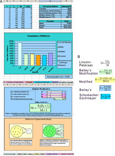
Figure 4. Histogram display (left) of estimates of population size and the equations (right) that underlie these estimates, from the spreadsheet program Mark–Recapture (Panks and Jungck, 2008).
A field activity on the mark–recapture method by Whiteley et al. (2007) was published in The American Biology Teacher. A free online module featuring five different mark–recapture models and a published data set on salamander populations (Panks and Jungck, 2008) is illustrated in Figure 4, A and B.
Game 3: Do You Get My Drift? (Population Genetics)
Because beanbag models of population genetics made this approach famous, there are many already available from diverse sources. The Froehlich and London (1996) exercise provides students with nine jars containing red and white beans in different proportions (10% red, 20% red, and so on). In each simulated generation, students draw five beans from the jar whose proportions matched their previous sample, until the population reaches fixation. In Barton's exercise (Barton, 2000), students pick tribeads out of boxes filled with plain beads of different colors to simulate not only genetic drift but also natural selection and some aspects of migration (gene flow). Both of these exercises are well structured and provide clear instructions for both learners and instructors. Access Excellence's Beans and Birds: A Natural Selection Simulation exercise (Access Excellence, 1995) simulates natural selection on a population of pinto beans in four different-colored backgrounds; however, this activity includes no explicit mathematics.
Some of our own computer simulations supplement these manipulatives. For example, Deme (Weisstein and Barnes, 2007) models the evolution of three local populations in response to natural selection, genetic drift, migration, and mutation (Figure 5). This general model can be modified to test specific evolutionary hypotheses from the primary literature. For example, researchers studying the CCR5Δ32 mutation, which substantially protects against HIV infection, proposed that this mutation might have conferred similar protection against bubonic plague (the Black Death) in fourteenth-century Europe. Using Deme, students can test this hypothesis by determining the fitness advantage required for the allele to reach its current frequency in a time frame consistent with published estimates of the allele's age.
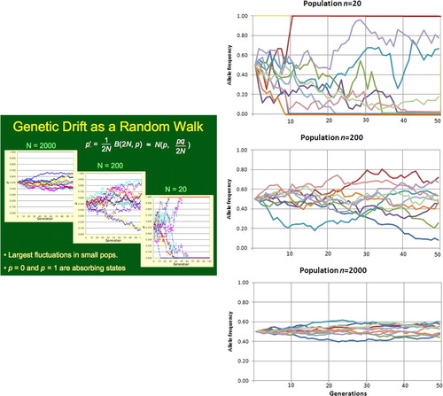
Figure 5. Left, genetic drift modeled with Deme (Weisstein and Barnes, 2007). Right, genetic drift modeled with software available under a Creative Commons license (Wikimedia, 2010). The simulations show genetic drift in populations of size N = 20, 200, and 2000, respectively. All populations start with allele frequencies of p = q = 0.5.
Our EVOLVE model (Soderberg and Price, 2003; Price et al., 2005) also simulates selection (parsed into reproduction and survival components), migration, and genetic drift. By gathering data on allele frequencies and population fitness, students can empirically test Fisher's fundamental theorem of natural selection (see Jungck, 1997). A similar model (Comar, 2005) focuses on mathematical methods, beginning with a model that uses only high school algebra and culminating in models that use ordinary differential equations.
Adding a third allele at the same locus yields an unexpected result: natural selection moves the population to its local fitness peak in the complex adaptive landscape but not necessarily to its global peak. Computer simulations such as deFinetti (Weisstein et al., 2005b) thus directly challenge the simplistic idea that selection produces “survival of the fittest” (Figure 6). Although the underlying mathematics relies on concepts from matrix algebra and partial derivatives, students with an understanding of high school algebra can easily follow the extension of the simple Hardy–Weinberg equilibrium equation to the one locus–three allele case.
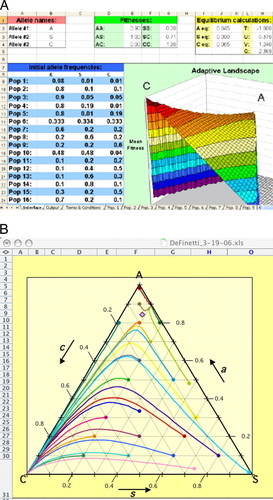
Figure 6. DeFinetti model of evolutionary fitness (top) landscape for one locus with three alleles and allele frequency trajectories (bottom) over 15 generations of selection (Weisstein et al., 2005b). These data are for modeling sickle-cell anemia with hemoglobin alleles A, C, and S. In the bottom image, populations near the AS polymorphism (top right) climb to their local peak rather than to the global peak (bottom left).
Game 4: Peas, Photons, and the Poisson Distribution
An exercise described by Buonaccorsi and Skibiel (2005) uses dried peas as manipulatives to introduce and test ecological hypotheses about the spatial distribution of individuals within a population. As they describe, “A Poisson distribution of split peas per sampling quadrat was generated as a student dropped a handful of split peas onto a grid that was projected on an overhead projector. Data analysis consisted of (1) tallying the observed frequencies of peas per quadrat, (2) calculating the mean number of peas per quadrat, (3) calculating the Poisson estimated probabilities for each outcome, (4) calculating the Poisson expected frequencies, (5) calculating and comparing the mean and variance of the distribution, (6) calculating the coefficient of dispersion (CD) and (7) evaluating the fit of observed and expected frequencies using a chi-square goodness-of-fit test. … From a biological viewpoint, schooling organisms (for example skipjack tuna) may exhibit clustered distributions whereas territorial competitive organisms may exhibit uniform or repulsed distributions (for example sea anemones).”
Berges (personal communication) converted this exercise into an analysis of photon absorption during photosynthesis. He reasons with students that most photons in sunlight will not be absorbed, due to reflection and scattering; as a result, absorption is a relatively rare and random event that can be modeled as a Poisson process (see Figure 7). His students have successfully modeled four species: tea, oak, maple, and aspen. In each case, as students increase the average number of lentils per square (a), the proportion 1 − P(0) of squares receiving at least one bean reaches an upper limit. This behavior mimics the saturation of photosynthetic output as a function of radiance. By fitting a rectangular hyperbolic curve to the resulting graph (Berges et al., 1994), students can estimate the density of gridlines on the sample surface, corresponding to the density of chlorophyll in individual species' chloroplasts. (Please consult Professor Berges for further specifics on this exercise.)
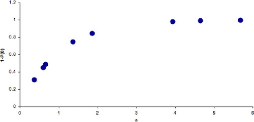
Figure 7. Results from one student simulation. As the average number of lentils per square (a) increases, the proportion of squares receiving at least one photon reaches an asymptotic maximum.
Berges's exercise uses the zero term of the Poisson distribution, P(0), to predict the proportion of chlorophyll molecules that do not receive any photons. This same term plays a key role in the Luria–Delbrück fluctuation experiment (Luria and Delbrück, 1943), one of the most famous experiments in twentieth-century biology. This experiment uses the number of plates with zero bacterial colonies to estimate the mutation rate (for an excellent historical analysis, see Zheng, 1999), and modified versions of the experiment also form the basis for many cancer models (e.g., Tlsty et al., 1989). The Luria–Delbrück experiment has been written up as both a wet lab exercise for undergraduates (Green and Bozzone, 2001) and a computer simulation that uses mean–variance tests for goodness of fit to the Poisson distribution (Weisstein et al., 2005a; Figure 8).
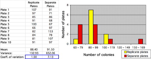
Figure 8. A screenshot from a computer simulation of the Luria–Delbrück experiment (Weisstein et al., 2005c). The histogram shows the distribution of plates with different numbers of bacterial colonies under two different procedures: replicate plates from a single growth culture (yellow bars) and individual plates from separate growth cultures (red bars). Because mutations may randomly arise at different times in different cultures, the latter procedure usually yields substantially greater variance in the number of colonies (blue), even when the mean number of colonies is roughly equal between treatments.
The same mathematical concepts can thus be used to study population ecology, photosynthesis, cancer, and bacterial mutation. Such examples help students understand the transferability of models across biological scales.
Game 5: Competition in a Cup
A central topic in mathematical biology education is the distinction between stochastic and deterministic models. The game FOXRAB (Moxley and Denk, undated) and its associated mathematical model allow students to explore these two different model types in the context of a predator–prey interaction. Although the formal Lotka–Volterra differential equations are beyond most beginning biology students, this simplified version captures most of the underlying dynamics while requiring only algebra at the high school level.
Each group of students is given one game board (Figure 9), 20 colored beans (rabbits), and 20 beans of a second color (foxes). Students mix this population thoroughly and then randomly distribute their beans on the board. The rules of FOXRAB are as follows:
When a rabbit lands on a black square, add another rabbit on that square (births).
When a fox lands on a white square, remove it (deaths).
When a fox lands in a patch of four squares that includes at least one rabbit, remove one of those rabbits (predation) and add a fox (birth).
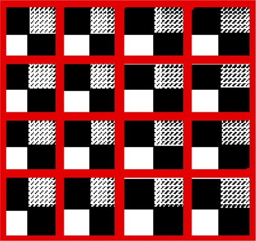
Figure 9. The FOXRAB game board is constructed from a checker- or chessboard, although it also can be constructed from a plain cardboard box. The 64 squares are divided into 16 patches of four cells each; we use colored tape to demarcate these boundaries.
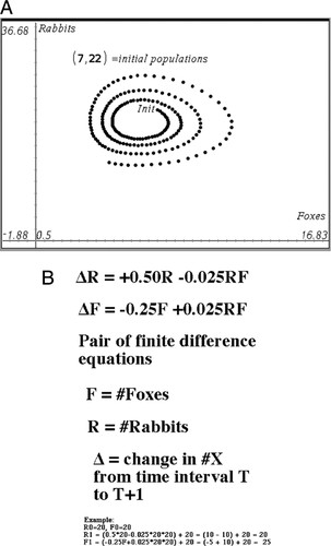
Figure 10. Top, phase portrait of foxes versus rabbits to examine for stable limit cycles (Hanna, 2010). Bottom, calculator tape for a pair of finite difference equations that fit the data from the board game quite well.
Once students have gained experience working with the physical game, we have them develop a simple set of recursion equations that combines births and deaths for each species (see Figure 10, bottom). These equations can easily be implemented on a hand-held calculator. At this stage, we contrast the stochastic behavior of the physical model, where each group gets different results due to random mixing and distribution of beans, with the deterministic behavior of the mathematical model. In particular, in what ways do the two models show similar behavior, and in what ways do they differ? We also ask students to devise modifications of the mathematical model so as to incorporate the stochasticity of real-world biological systems.
Both FOXRAB and the calculator-based model become tedious to run for >10 generations. Once students have used these tools to build their intuitive understanding of how the system works, we introduce them to a software package such as Two-Species Model (Weisstein et al., 2005c), which can quickly produce larger data sets. We then shift students' attention from the model mechanics to more fundamental questions about population dynamics. For example, although most students can correctly interpret simple X-Y scatterplots of rabbits and foxes versus time, they struggle to understand phase portraits of foxes versus rabbits (Figure 11), in which time becomes an embedded variable. Students also become interested in the short-term oscillations that can arise within each species in a discrete model of logistic growth and in the chaotic behavior produced by rapid population growth.
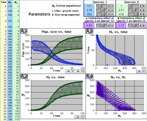
Figure 11. Screenshot from the Two-Species Model software tool (Weisstein et al., 2005c), showing competitive exclusion of one species (blue) by another (green). Both populations' high growth rate leads them to repeatedly overshoot their carrying capacity and then die back, producing oscillations of period 2. Graph A4 (purple, bottom right) is a phase portrait plotting the population size of species 2 (y-axis) versus the population size of species 1 (x-axis).
Game 6: One Good Urn: How a Game Changes Our Expectations
In 1976, Joel Cohen (Cohen, 1976) coined the phrase “one good urn” to describe the following beanbag experiment (Figure 12):
“Suppose a very large box … contains one green ball and one blue ball. Choose one ball at random, look at its color, replace the ball in the box, and add to the box another ball of the same color as the one chosen. At each successive point in time, say once every second, choose one ball at random and then repeat exactly the above …
“What will happen to the proportion of green balls as time increases? … The experiment just described is a special case of what is known as “Pólya's urn scheme.” Eggenberger and Pólya (1923) introduced the scheme to model the spread of infection in a population.… [T]he limiting distribution of proportions of each color is uniform.”
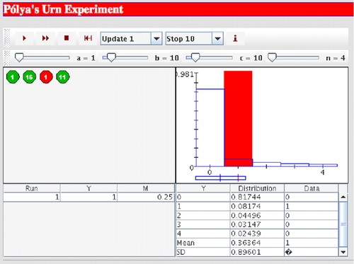
Figure 12. Screenshot of a computer applet (Siegrist, 2009) that demonstrates the Pólya urn experiment. After each trial, the applet displays the number and proportion of red balls, as well as the corresponding probability density function. A similar interactive tool is available through the Wolfram Demonstrations Project (Hennings, 2010).
Lou Gross, the head of the National Institute for Mathematical Biology Synthesis Center (NIMBioS), regularly demonstrates this game at conferences. Initially, most participants predict that the frequencies of each color will fluctuate randomly over time. During the experiment, most participants' cups begin to drift toward a preponderance of one color or the other, and participants often revise their prediction accordingly. Once the experiment is complete, however, combining data across all participants reveals a uniform distribution: all physically possible proportions of green vs. blue beads are equally likely. Comparing participants' initial predictions to their results reinforces a final feature of manipulative models: the ability to surprise. A seemingly simple game can yield insight into counterintuitive results that students would otherwise reject as implausible. Much like the magician showing how a trick is done, manipulatives help explain the unexplainable.
CONCLUSIONS
The reprinting of Haldane's paper defending the use of beanbag models in population genetics has led to further discussion of both the utility and the limitations of such models. For example, Kraft and Raychaudhuri (2009) note the following:
“Haldane conceded this point of principle (beanbag genetics do not explain the physiological interaction of genes and the interaction of genotype and environment) but went on to argue that despite its simplifications, the marginal approach had proven itself in practice and led to important insights. The arrival of massive amounts of data from genome-wide association studies (GWAS) has turned up the heat on a similar debate in the field of genetic epidemiology. On the one hand, the admittedly simple approach of averaging over genetic and environmental backgrounds and testing each marker in a GWAS for association with the studied trait marginally has proven quite successful, despite early concerns that by ignoring the underlying complexity this naïve approach would fail. On the other hand, the loci discovered to date do not come close to explaining the observed heritability for most studied traits. Pathway analyses acknowledge complexity by considering multiple loci simultaneously and relating them to known functional annotations.”
Kraft and Raychaudhuri (2009) note that data mining approaches can be used to untangle the complex interactions that Mayr had originally emphasized. Thus, in some sense, current work in genetic epidemiology is coming full circle by integrating Haldane's beanbag approaches with Mayr's views on the complexity of real genetic systems.
To illustrate the breadth of these issues, in the 2009 issue of Judgment and Decision Making, neurobiologist Benjamin Hayden and evolutionary anthropologist Michael Platt use the example of the St. Petersburg paradox (Hayden and Platt [2009]; Figure 13) to underscore the fundamental differences between the mean and the median. In the St. Petersburg game, the player tosses a fair coin repeatedly until a tail first appears. The player then wins 2n dollars, where n is the number of consecutive heads tossed by the player. Although this game has an infinite expected payoff (mean), the median payoff is only one dollar. Hayden and Platt (2009) suggest that decision makers dealing with high-risk situations intuitively use medians instead of means, due to the latter's lability and susceptibility to outliers. As a result, they may not plan sufficiently for low-probability, large-magnitude events (e.g., the current oil spill in the Gulf of Mexico). Simple beanbag models and games thus not only provide learning tools for students but also inform decisions by contemporary scientists and policy makers in diverse fields.
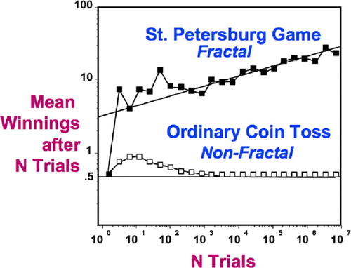
Figure 13. Model of the St. Petersburg game (from Leibovitch, 1998). Because the payoff doubles with each successful coin toss, the player's mean winnings increase with the number of trials. This process is driven primarily by rare but extreme events (e.g., tossing 10 heads in a row).
Thus, as Borges (2008) concludes, “Despite all these assaults, the beanbag endures, with the formulation of better and more sophisticated theoretical population genetics models that include multiple interacting loci, thus making the transition from the classical models of Fisher, Wright and Haldane to more modern ones. Surely as long as evolutionary biologists need to explore the realms of the possible versus the actual, the beanbag will live on.”
ACKNOWLEDGMENTS
We thank many colleagues in the BioQUEST Curriculum Consortium. Numerous participants in workshops helped us develop and refine materials and strategies. Funding from several National Science Foundation grants over the years from the National Science Digital Library (both American Association for the Advancement of Science's BioSciEdNet and Mathematical Association of America's Mathematical Sciences Digital Library) and the CCLI undergraduate program have been enormously helpful in being able to offer workshops and share materials developed online. A grant from Dr. Claudia Neuhauser from her Howard Hughes Medical Institute Professorship at the University of Minnesota has been especially appreciated as well as the opportunity to learn from her Numerical Undergraduate Mathematical Biology Education … [NUMB3R5 COUNT]) project. Similarly, the financial and personal support provided by Dr. Lou Gross, Director of NIMBioS, has been invaluable. Larry Leibovitch, Associate Dean for Graduate Studies & Programs, Charles E. Schmidt College of Science, Florida Atlantic University, has shared wonderful examples of manipulatives in mathematical biology through his presentations, articles, books, website, and personally to us. John Berges, Chairperson, Biology, University of Wisconsin Milwaukee, generously shared lentil photosynthesis activity and analysis.


