Probabilities and Predictions: Modeling the Development of Scientific Problem-Solving Skills
Abstract
The IMMEX (Interactive Multi-Media Exercises) Web-based problem set platform enables the online delivery of complex, multimedia simulations, the rapid collection of student performance data, and has already been used in several genetic simulations. The next step is the use of these data to understand and improve student learning in a formative manner. This article describes the development of probabilistic models of undergraduate student problem solving in molecular genetics that detailed the spectrum of strategies students used when problem solving, and how the strategic approaches evolved with experience. The actions of 776 university sophomore biology majors from three molecular biology lecture courses were recorded and analyzed. Each of six simulations were first grouped by artificial neural network clustering to provide individual performance measures, and then sequences of these performances were probabilistically modeled by hidden Markov modeling to provide measures of progress. The models showed that students with different initial problem-solving abilities choose different strategies. Initial and final strategies varied across different sections of the same course and were not strongly correlated with other achievement measures. In contrast to previous studies, we observed no significant gender differences. We suggest that instructor interventions based on early student performances with these simulations may assist students to recognize effective and efficient problem-solving strategies and enhance learning.
INTRODUCTION
Most core undergraduate science curricula contain associated laboratory or discussion sections. The main goal of these sections is to extend the lecture material through activities that integrate course content and promote the students' critical thinking and problem-solving skills. These activities take many forms, including hands-on wet-lab activities, paper discussions, peer-directed and collaborative assignments, computer-based assignments, and so forth.
A recurring challenge for instructors in these settings is determining whether the students are indeed learning to think critically as well as mastering the content. While a variety of qualitative and qualitative tools/approaches are available which provide summative measures of overall student learning (Sundberg, 2002; Tanner and Allen, 2004), few provide detailed insights into the dynamics of strategy and skill formation as students gain problem-solving experience (Alexander, 2003).
This suggests that if dynamic models of how students approach and solve scientific problems could be created, they could be important formative assessment tools. For instance, such models could document and begin to explain the diversity of learning approaches of individual students and student groups (for instance, across gender). They could also help guide more uniform learning experiences for students across discussion sections, by documenting the qualitative and quantitative strategic differences employed in different setting or with different instructors. Such analyses could also provide real-time assessment of classes in progress and help identify candidates for intervention. Finally, if sufficiently detailed, such models could be predictive of students' future performances and used to evaluate the effectiveness of various learning supports.
Learning trajectories describe the differences between novices and experts in a problem-solving task. Novices often have limited and fragmented knowledge that contributes to a lower ability to “frame the problem,” that is, recognize the importance of problem elements and prioritize solution strategies. Novice strategies are often ineffective (they fail to reach the correct answer) and inefficient (they require more steps, more time, more reference material). Experts are more efficient in the use of resources and deriving the correct answer. These can be viewed as defining stages of understanding as experience is developed (VanLehn, 1996). With practice, students' knowledge becomes more structured and deeper, and this is reflected by changes in their strategic approaches. Eventually most students adopt an approach with which they are comfortable that they will use for similar types of problems in the future. Although it is apparent that most students do not continually improve on most tasks, there are few descriptions as to how and why individuals differentially stabilize their performance levels.
In this article, we build on these ideas and describe a process for developing probabilistic models of problem solving based on students' performance on a series of online microbial genetics simulations. In constructing frameworks for these models, we felt they should 1) reflect what students do, 2) be able to categorize rapidly each performance with regard to the adequacy of the strategic approach, 3) provide a measure and benchmarks for progress, and 4) be easy to understand and relate to other performance measures. We describe this modeling approach for molecular genetics, but it is applicable to many domains in which scientific competence is being developed.
TASK AND METHODS
Problem-Solving Task
The online software used for these studies, termed IMMEX (Interactive Multi-Media Exercises), has been useful for understanding how strategies are developed during scientific problem solving (Stevens et al., 1999; Underdahl et al., 2001). IMMEX problem sets, which follow the hypothetical-deductive learning model of scientific inquiry (Lawson, 1995; Olson and Loucks-Horsley, 2000) are created by teams of educators, teachers, students, and university faculty and are aligned with discipline learning goals and state and national curriculum objectives (Stevens and Palacio-Cayetano, 2003). In these online scenarios, students are expected to frame a problem from a descriptive scenario, judge which information is relevant, plan a search strategy, gather information, and eventually reach a decision that demonstrates understanding. These exercises are closed-ended; that is, they work from a specific starting point and work toward a single correct answer.
We have used the IMMEX problem set The lac Operon, which focuses on the expression and regulation of bacterial genes, to develop learning trajectory models (Johnson et al., 2004). This and other IMMEX problems can be explored at the IMMEX home site: http://www.immex.ucla.edu. The scenario begins with a student being given a strain of Escherichia coli with a mutation in the lactose operon and the task is to determine the location of this mutation. There are menu items available for laboratory data such as indicator plates, enzyme assays, protein or RNA expression blots, gene maps, as well as glossary references to these techniques that provide explanations (Figure 1).
By clicking on these menu items, students can get specific test results, and when the item is selected, they are shown a brief multimedia presentation of the test being performed and directly observe the results. The IMMEX database collects timestamps of these action items when the student makes the selections.
To ensure that students gain adequate experience, this problem set contains six cases that can be performed in class, assigned as homework, or used for testing. These cases, 1-6, represent the mutations 1-6 in Figure 1. Interestingly, case 2 was significantly (Pearson χ2 = 122.4, p, .000) more difficult, with a solved rate of 59% compared with the other five cases, which have a solved rate of 80%.
Classroom Setting
The discussion sections where The lac Operon problem set has been implemented were weekly, 1-h classes of ∼25 students. They were designed to review the lecture material of the previous week and, as much as possible, help students develop critical thinking skills in molecular biology. The problem-solving software component consists of two IMMEX problems, Which Plasmid Is It?, which provides experience in DNA restriction mapping, and The lac Operon. The specific assignment for the 2003 classes was to have the students do all six lac Operon cases, and 360 students participated. In the summer 2003 class, the IMMEX problems were optional, only five lac Operon cases were required, and 160 students participated. In the 2004 classes, the assignment was to complete five cases, and 256 participated. Thus, a total 776 students completed 3,599 cases that were further subjected to analysis. In all classes, the first two cases were not graded, allowing the students use these attempts to acquaint themselves with the problem space. The final three cases were scored based on whether the student solved the case or not (5 points for solving the problem on the first attempt, 4 points for solving it on the second attempt, and fewer points for not getting a correct answer). Of the students who participated in this exercise in 2004, the average score was 12.4 out of 15 possible, suggesting that the students took the assignment seriously.
Sources of Performance Data
In constructing and validating our model of student learning, we have relied on the following pieces of summative evidence:
Student summaries of their problem-solving approach
Problem-solving data from six The lac Operon cases
Discussion section grades
Overall course grades
The modeling approaches and tools we used included the following:
Categorization of common strategies by artificial neural network clustering
Models of learning progress derived from hidden Markov modeling
For this article, we detail the performances of three students that represent high (student 86588), medium (student 86525), and low (student 86763) overall performance in the discussion sections. The performance and modeling data for these students are shown in Appendices A, B, and C.
Student Summaries
To stimulate meta-cognition and provide evidence of strategic thinking, students could write, for 5 extra credit points, a short (one paragraph) essay on “My Winning IMMEX Strategy.” This assignment was optional in 2004, and 136 essays were received. The assignment was mandatory in 2003, and 305 essays were received.
Figure 1. The lac Operon. In The lac Operon problem set, students access a variety of assays used in a molecular biology laboratory to determine the location of the structural and regulatory mutations within the lactose operon of Escherichia coli.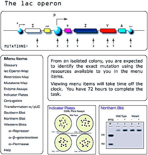
The three essays of the highlighted students (86588, discussion grade 9.5; 86525, discussion grade 7.5; 86763, discussion grade 6.5) suggest that students adopt hypothesis-testing approaches of different degrees of diversity and structure. The first student developed a hierarchical if-then approach; the second, a more limited approach focusing on structural rather than regulatory aspects; the third, a strategy focused on one test category. The first student appeared to spend time early to understand mutations, the lactose operon structure, and the different techniques available, whereas the other two students did not mention this process. By investing time to frame the problem, this student was adopting a strategy more like experts, who proportionally spend more time in framing a problem than do novices (Chi et al., 1988). This problem-framing process helps keep the complexity within manageable dimensions for the student and would be expected to lead to improved future performance (King and Kitchener, 1994; Lynch, 2000).
Search Path Maps of Student Performances
We first wished to determine how these student statements encapsulated what they actually did. For this, we used online visualization technologies that trace the sequence of item selections by students (Stevens, 1991). The lac Operon problem space contains 41 data items (available as buttons) that students view in any order they feel appropriate and that contain the information needed to solve the case. We create visual representations, or templates, of the problem space where related conceptual items are grouped together and color coded. We then use a series of lines to connect the sequence of items selected. Some of the search path maps can become complex as students transit the problem set (Figure 2).
A comparison of the search path maps with the student essays indicated a close correspondence. For instance, student 86525 verbalized the selection of enzyme assays and protein blots as core parts of his or her strategy, and this is also shown by the search path maps. From these maps, it is also apparent that with practice the student strategies changed, becoming more efficient (i.e., fewer tests), more rapid, and, for the most part, more effective.
Figure 2. Sample Search Path Map. The first performance of student 86588 has been overlaid on the The lac Operon template with lines connecting the sequence of test selection. For this problem template the green items are in the Glossary, the yellow items are enzyme assays, DNA and RNA blots are orange, the mutation and restriction maps are red, the protein blots are purple, and the conjugation/transformation assays are pink. The lines go from the upper left-hand corner of the “from” test to the lower center of the “to” test. Items not selected are shown in transparent gray. At the top of the figure are the overall statistics of the case performance. At the bottom of the figure is a time line on which the colors of the squares link to the colors of the items selected, and the width of each rectangle is proportional to the time spent on that item. These maps are immediately available to teachers and students at the completion of a problem.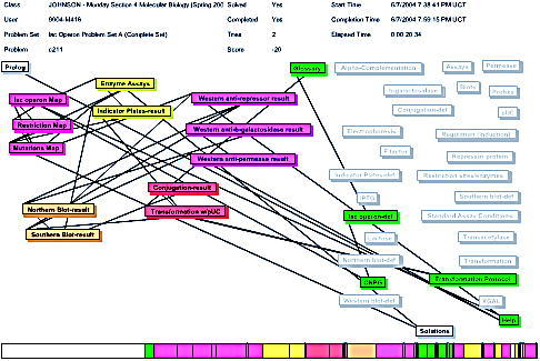
These maps are available for all students and their teachers in real time on the Web following completion of a case. Students may have used them to write their essays, which were then used to stimulate class discussions of efficient and inefficient strategies. Although informative, these maps can be time consuming to group, given a class of 256 students. To overcome this limitation, the next step in our modeling uses artificial neural networks (ANN) to identify and categorize the most common approaches.
Defining Strategies with Artificial Neural Networks
ANNs derive their name and properties from the connectionist literature, share parallels with the theories of predicted brain function (Rumelhart and McClelland, 1986) and have properties that make them attractive candidates for modeling learning trajectories (Stevens and Casillas, 2004; Stevens and Najafi, 1993; Stevens et al., 1996).
Rather than being programmed per se, the neural networks build internal models of complex processes through training routines in which thousands of examples of the process being modeled are repeatedly presented to the software. When appropriately trained, neural networks can generalize the patterns learned to encompass new instances and predict the properties of each exemplar. Relating this to student performance of online simulations, if a new performance (defined by sequential test item selection patterns) does not exactly match the exemplars provided during training, the neural networks will extrapolate the best output according to the global data model generated during training. For performance assessment purposes, this ability to generalize is important for “filling in the gaps” given the expected diversity between students with different levels of experience.
The mathematics behind self-organizing neural networks is such that groups of similar performances appear on an output 6 3 6 grid of classifications as physically near each other (Kohonen, 2001). ANNs yield a “topological map” of similar performances on which the geometric distance between nodes is a metaphor for similar solving strategies. The search path map for the first, second, and sixth performances of student 86588 are quite different and clearly separated by the ANN (refer to Appendices). Similarly, the third performance of students 86588 and 86525 appear similar to the eye and cluster together on the ANN nose map.
For these studies, we used a 36-node neural network that was trained with 2,564 performances of The lac Operon derived from university students, and most students performed five or all six cases in the problem set. Choices regarding the number of nodes and the different architectures, neighborhoods, and training parameters have been described previously (Stevens et al., 1996).
To understand the basis of this classification, the organization of strategies from the trained neural networks were visually represented at each node of the neural network by histograms showing the frequency of items selected by students (Figure 3). For The lac Operon, there are 41 items that relate to Glossary Information (items 2-27), Molecular Maps (items 28-30), Enzyme Assays and Transformations (items 31-35), and RNA, DNA and protein blots (items 36-40). Item 41 was a worksheet that students could print out to take notes. The resulting 36 classifications are variables that can be used for immediate feedback to the student, serve as input to a test-level scoring process, or serve as data for further research by linking to other measures of student achievement as we show later in this article.
Figure 3. Sample nodal analysis. This nodal analysis diagram shows the frequency with which each item was selected during the performances at the particular node (node 9). The associated labels identify general categories of these tests.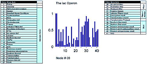
Most strategies defined in this way consist of items that are always selected for performances at that node (i.e., those with a frequency of 1) as well as items that are ordered more variably. For instance, all Node 9 performances shown in Figure 3 contain the items 1 (Prologue) and 2 (Glossary). Items 22, 29-31, and 38 have a selection frequency of 60%-80%, and thus any individual student performance would most likely contain only some of these items. Finally, there are items with a selection frequency of 10%-30%, and we regard these more as background noise, rather than a significant contributor to a strategy. Figure 4 is a composite nodal map, which displays the strategic topology generated during the self-organizing training process
Given that the neural network was trained with vectors representing the items that students selected, it is not surprising that a topology is developed based on the quantity of items. For instance, the middle of the first row of the map (node 4) represents strategies where a large number of tests are being ordered, whereas the lower left contains clusters of strategies where few tests are being ordered. Differences reflecting the quality of information being accessed are also easily seen. An example of a general qualitative strategic difference is where students select a large number of items, but no longer use the Glossary. These strategies are represented on the right-hand side of Figure 4 (nodes 6, 12, 18, 24, 30, and 36) and are characterized by extensive selection of items mainly on the right-hand side of each histogram. Nodes 2, 8, and 14 illustrate another qualitative difference in which there is predominantly a usage of enzyme assays.
Once ANNs are trained and the strategies represented by each node are defined, new performances can be tested on the trained neural network, and the strategy (node) that best matches the new input performance vector can be identified. For instance, were a student to order many glossary items and tests while solving a The lac Operon case, this performance would be classified with the nodes of the upper center of Figure 4, at node 4, whereas a performance where the mutation maps were reviewed followed by gene expression assays would be more toward the center or the lower-left corner. The strategies defined in this way can be aggregated by class, grade level, school, or gender and related to other achievement and demographic measures.
For instance, the ANN category of each of the performances of the three students described here is shown in Table 1. Students 86588 and 86763 started with a similar strategy that included the examination of most of the data; student 86525 showed a leaner strategy by not examining the nucleic acid blots or the conjugation and transformation assays. By the third case, student 86525 had adopted a strategy that included mutations maps, enzyme assays, Western blots, and Southern blot. Student 86763, although slowly stabilizing on an approach dominated by looking at all maps and performing all Western blots, continued to vary his or her strategic approach by continual reference to the glossary material. Through such inspections, the student performances shown by the search path maps can begin to become described in terms of nodal categories.
| Example | Strategy Sequence | Description | ||||||||||
|---|---|---|---|---|---|---|---|---|---|---|---|---|
| 86588 | 6 | 34 | 20 | 18 | 32 | 20 | Many tests initially, with decreased use of blotting techniques with experience | |||||
| 86525 | 23 | 12 | 20 | 29 | 29 | 29 | Progressive refinement and stabilization of a strategy consisting of restriction maps and blotting techniques | |||||
| 86763 | 6 | 9 | 16 | 22 | 9 | 23 | Many test selections | |||||
Defining Progress with Hidden Markov Models
ANN analyses provide point-in-time snapshots of students' problem solving. More complete models of student learning include changes in student strategies with practice. A novice learner might choose to review all available data items. The same strategy in a more experienced student would indicate a lack of progress, because a more experienced learner would be expected to choose only pertinent data items. More complete models of student learning therefore have to take into account the changes of student's strategies with practice.
Figure 4. Complete The lac Operon Neural Network Topology Map. Following training with 2,240 student performances, test usage histograms were created for each node showing the frequency of action items selected at each of the 36 nodes. The proportion of the dataset clustered at each node is shown above each figure.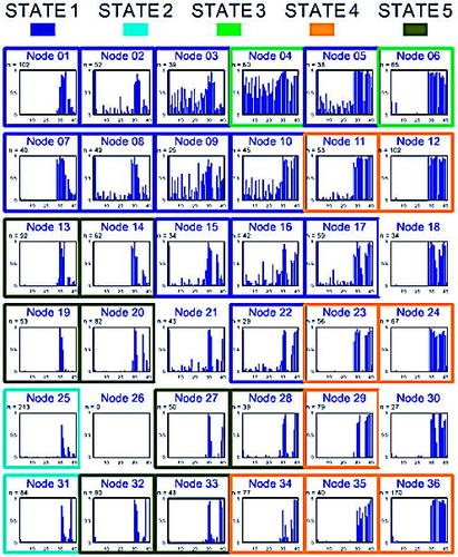
Figure 5. A Markov chain showing the probability that Hal (the robot) will enter various rooms.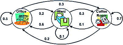
In this research we have used hidden Markov modeling to extend these preliminary results to more predicatively model student learning pathways. Markov models are used to model processes that move stochastically through a series of predefined states (Rabiner, 1989). The states are not directly observed but are associated with a probability distribution function. For example, imagine a robot, whom we will call Hal, that wanders through a hospital from room to room performing various duties. Hal's virtual map might include a doctor's office, a ward, and the coffee room. The arcs in a Markov chain describe the probability of moving between states, and the sum of the probabilities on the arcs leaving a state must sum to one. So, in Figure 5, we see that if Hal is in the doctor's office, there is a 20% chance that he will move to the ward, a 30% chance that he will wander to the coffee room, and a 50% chance that he will just stay put. Markov chains also specify that the probability of a sequence of states is the product of the probabilities along the arcs. So, if Hal is in the doctor's office, then the probability that he will move to the ward, and then the coffee room is (.2)(.3) = .06, or 6%.
Hidden Markov models generalize Markov chains in that the outcome associated with passing through a given state is stochastically determined from a specified set of possible outcomes and associated probabilities. Consequently, it is not possible to determine the state the model is in simply by observing the output (i.e., the state is “hidden”). For example, we might estimate Hal's location (state) by an account of the messages displayed on his chest (outcomes). A given sequence of observations may be associated with more than one possible path through the hidden Markov model. The observation symbol probability distribution describes the probabilities of each of the observation symbols, for each of the states, at each time.
Hidden Markov modeling methods have been used successfully in previous research efforts to characterize sequences of collaborative problem-solving interaction, leading us to believe that they might show promise for also understanding individual problem solving (Soller, in press; Soller and Lesgold, 2003). Interested investigators might visit: http://www.ai.mit.edu/~murphyk/Software/HMM.
In applying this process to model student performance, a number of unknown states are postulated to exist in the data set that represent strategic transitions that student may pass through as they perform a series of IMMEX cases. For most IMMEX problem sets, a postulated number of states between 3 and 5 have produced informative models. Then, similar to ANN analysis, exemplars of sequences of strategies (ANN node classifications) are repeatedly presented to the hidden Markov modeling software to develop progress models. These models are defined by a transition matrix that shows the probability of transiting from one state to another, an emission matrix that relates each state back to the ANN nodes that best represent that state, and a prior matrix that postulates the most likely starting states of the students.
The transition matrix for The lac Operon hidden Markov model is shown in Table 2. By looking along the diagonal (bold), States 2, 4, and 5 appear stable, suggesting that once a student adopts a strategy represented by these states, her or she is likely to remain there. In contrast, students adopting State 1 and 3 strategies are less likely to persist with those states but are more likely to adopt other strategies (gray boxes).
| To State | |||||||||
|---|---|---|---|---|---|---|---|---|---|
| From State | 1 | 2 | 3 | 4 | 5 | ||||
| 1 | 0.685 | 0.042 | 0.017 | 0.005 | 0.249 | ||||
| 2 | 0.000 | 0.999 | 0.000 | 0.000 | 0.000 | ||||
| 3 | 0.315 | 0.163 | 0.183 | 0.225 | 0.111 | ||||
| 4 | 0.000 | 0.002 | 0.000 | 0.965 | 0.032 | ||||
| 5 | 0.000 | 0.055 | 0.000 | 0.000 | 0.944 | ||||
The emission matrix resulting from the trained hidden Markov model also provides the probability of any particular node (emission) occurring in any particular state. In addition to providing the test selection composition of each node, Figure 4 also has been color-coded to show the most likely state that each node is associated with. Here State 3 consists of nodes 4 and 6 in the upper right corner, and State 5 contains nodes predominantly in the lower-left portion of the ANN grid. Table 3 summarizes the properties of each of the states with respect to the items selected and the solve rate.
| State | Solve rate (%) | Transitions | Items represented |
|---|---|---|---|
| 1 | 75 | In transit | Maps, enzymes, and limited blots |
| 2 | 76 | Stable | Enzyme assays and very limited other tests |
| 3 | 62 | In transit | Mostly test items and descriptions |
| 4 | 75 | Stable | All maps, all enzymes, and all blots |
| 5 | 85 | Stable | Effective testing—limited use of enzymes and blots |
Finally, Table 4 shows the prior probabilities derived from the hidden Markov model. This indicates that the most likely state for students to begin in on their first The lac Operon performance is State 3, followed by states 2 and 4.
| State | Prior probability |
|---|---|
| 1 | .01 |
| 2 | .03 |
| 3 | .69 |
| 4 | .15 |
| 5 | .12 |
RESULTS
The modeling approach described here results in a model in which 1) each new performance can be categorized into one of 36 groups and 2) a series of performances can be grouped into one of five sequences with probabilities of transiting from each state to another.
In this section we begin to explore the validity, usefulness, and limitations of this modeling process by asking questions such as the following:
What is the diversity of student strategies?
How do strategies change with practice?
Are there multiple learning trajectories?
Do different classrooms share similar learning trajectories?
Are there gender differences in how students approach and solve problems?
How does IMMEX problem-solving performance compare with summative assessments?
Case Specificity of ANN Nodal Categories
We first examined the case specificity of each of the categories defined by the ANN analysis; that is, cases were analyzed individually rather than as a group of all six. Certain nodes were significantly enriched for performances of different cases. For instance, cases 1 and 3 where the mutations were in the repressor and operator genes showed an enrichment of performances at nodes 31 and 32. Here, in addition to the mutations map and enzyme assays, all students at this node also selected an antirepressor protein Western blot. Similarly, the performances for case six, the permease mutation, were enriched at nodes 21 and 27, and included the Western blot for permease enzyme.
Case 2, the promoter mutation and the most difficult case in the problem set, showed a different form of case specificity with higher than expected numbers of performances at nodes 11, 12, 17, and 18. These nodes represent strategies for which almost all of the data available are being accessed, suggesting, perhaps, that students were solving this case by a process of elimination rather than confirmation. Student feedback suggests that unexpected data was confusing. Specifically, students expected the mutation to ablate promoter activity completely, whereas in Case 2, some residual activity remained.
Interestingly, the case specificity only applied when the solved performances were examined, indicating that for The lac Operon there are relatively few ways to solve each problem, but many ways to miss them.
Gender
The male and female students in the discussion section performed the same number of cases and solved the same proportion of cases (Pearsonχ 2 = 3.8, p. .05). A two-way contingency table analysis was conducted to evaluate whether male and female students were differentially using strategies represented by the ANN nodes or the hidden Markov model states. Unlike other problem sets we have examined (Stevens et al., in press), there were no differences in strategies employed by the two groups.
Solution Frequencies and Learning Trajectories
The overall solution frequency for The lac Operon testing data set (N = 3,599 performances) was 76%, and there were significant solved rate differences between the states (Pearson χ2 = 79.2, p < .000). State 3, which is characterized by exhaustive use of data and descriptive items, had a lower than average solve rate, and State 5, which is characterized by limited and efficient use of data items, had a higher than average solve rate (Table 3). The solve rates at each state provided an interesting view of progress. For instance, if we compare the differences in solve rates shown in Table 3 with the most likely state transitions from the matrix shown in Table 2, we see that most of the students who start at State 3, and have the lowest problem solving rate (62%), will transit either to States 1 or 4. Those students who transit from State 3 to either State 1 or State 4 will show, on average, a 15% performance increase. The students at State 4, however, are most likely to maintain their strategies (using most of the enzyme assays and blots), whereas those in State 1 have a high probability of transiting to State 5, which is the most efficient problem solving state.
Dynamics of State Changes
Over the course of 6 The lac Operon performances, the solved rate increased from 67% (case 1) to 80% by case 3 (Pearson χ2 = 46.8, p < .000), and this was accompanied by corresponding state changes (Figure 6). These changes over time were characterized by a decrease in the proportions of States 1 and 3 performances and increases in States 2, 4, and 5 performances.
Figure 6. Changes in HMM State Distributions with Experience. This bar chart tracks the changes in all student strategy states across six The lac Operon performances. Mini-frames of the strategies in each state are shown for reference.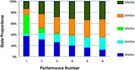
Problem-Solving Ability and State Transitions
Learning trajectories were then developed according to students' overall problem-solving ability as determined by item response theory analysis (Linarce, 2001). This analysis is similar to the overall solve rate for a student, but it also factors in the performance of each student on each case, thus accounting for the difficulty of the cases. The data is usually expressed in terms of a person measure, which ranges from 0 (lowest) to 100 (highest). For these studies, students were grouped into high (person measure = 72-99), medium (person measure 50-72), and low (person measure 20-50) categories. There were significant state differences between the different groups (Pearsonχ 2 = 68.3, p < .000) with the highest group (group 3) showing a larger than expected use of State 5, the intermediate group (group 2) showing higher than expected use of State 4, and the lowest group (group 1) showing a higher than expected use of States 2 and 4. These data indicated that students with different problem-solving abilities were employing different strategic approaches as they problem solved across the six lac Operon cases. As shown in Figure 7, the state distributions of the students in the different groups changed little after the fourth case, suggesting that additional practice alone would not turn low-performing students into higher-performing students.
Learning Trajectory Differences across Classrooms
Learning trajectories were then examined across different classrooms. Although there we no significant differences in the solved rates across classrooms (Pearson χ2 = 21.3, p = .049), there were large differences across classrooms in the nodal categories (Pearsonχ 2 = 1877, p < .000) and hidden Markov model states (Pearson χ2 = 465, p < .000). Four representative classrooms are shown in Figure 7 that exhibited different starting state distributions, final state distributions, or both. Some classrooms rapidly adopted effective problem-solving strategies (i.e., States 4 and 5 for class 2202), whereas other classes were slower in developing an effective learning trajectory (i.e., class 2203).
Correlation with Other Measures
A final set of studies related the students' overall problem-solving ability with other course assessments including the overall course grade and the discussion section grade. This was conducted for the year 2004 students for whom the summative grades were available. The overall course grade consisted of a midterm examination, a discussion section grade, and a final examination. The discussion sections and lectures are run independently, so material unique to the discussion section will not be explicitly covered on the examinations, which consisted of standard short answers and essays. As shown in Table 5, the correlations between overall problem-solving ability, the final examination, and discussion section grades were moderate.
| Problem solving | Discussion | Final | |
|---|---|---|---|
| Problem solving | |||
| Pearson correlation | 1 | .494** | .286** |
| p (two-tailed) | .000 | .000 | |
| Discussion | |||
| Pearson correlation | .494** | 1 | .608** |
| p (2-tailed) | .000 | .000 | |
| Final | |||
| Pearson correlation | .286** | .608** | 1 |
| p (2-tailed) | .000 | .000 |
A more detailed study was then performed across discussion sections using the discussion section grade along. The discussion section grade represented 10% of the total course grade and was determined from three quizzes, each worth 25 points, and the homework, which also accounted for 25 points of the final grade. As shown in Table 6, the correlation between these measures was variable across these classes ranging from very high correlations (classes 2202, 2203, and 2207) to no correlation (classes 2205, 2208, 2210, and 2200). Interestingly, these could not be explained by overall problem-solving or discussion grades across the classes, which were not significantly different.
| Class ID | Problem solving | Discussion | N | r | p values |
|---|---|---|---|---|---|
| 2202 | 68 | 72 | 76 | .874 | 0 |
| 2203 | 70 | 68 | 98 | .714 | 0 |
| 2205 | 71 | 73 | 95 | −.040 | .711 |
| 2206 | 72 | 73 | 157 | .513 | 0 |
| 2207 | 67 | 67 | 110 | .761 | 0 |
| 2208 | 66 | 61 | 115 | −.020 | .840 |
| 2209 | 72 | 69 | 124 | .321 | 0 |
| 2210 | 57 | 64 | 146 | .276 | .001 |
| 2211 | 68 | 77 | 121 | .564 | 0 |
| 2200 | 65 | 64 | 127 | .133 | .135 |
DISCUSSION
There were several goals of this study. The first was to develop models of how students gain competence in domain-specific problem solving. We were particularly interested in learning whether the combination of ANN analysis for describing a performance and hidden Markov modeling for describing progress across a sequence of performances resulted in useful models of the learning trajectories being explored. Next, we wished to understand the factors influencing student's position and progress along the framing, transitions, and stabilization stages of the learning trajectory for The lac Operon.
In relating our models to a learning trajectory framework, the early framing stage where strategies are being formulated was best represented by State 3. From the prior probabilities matrix from hidden Markov modeling training, these are the strategies that students are most likely to adopt on their first lac Operon case (probability = .69) and is also represented by students extensively exploring the problem space and selecting most of the experimental data as well as multiple glossary items. As expected, the solved rate for this state was the lowest, suggesting that State 3 strategies represent the more surface-level strategies, or those built from situational (and perhaps inaccurate) experiences. From the transition matrix, State 3 is not an absorbing state and most students move from this strategy type on subsequent performances. It is likely that State 3 contains subsets of students containing those that 1) will explore extensively on the first case and then rapidly leave it and 2) those who tend to persist longer with this approach.
Figure 7. Learning Trajectories For Students With Different Abilities. The individual student population was separated into different ability levels as described in the Methods section and the strategy state usage was determined for each of the six The lac Operon performances.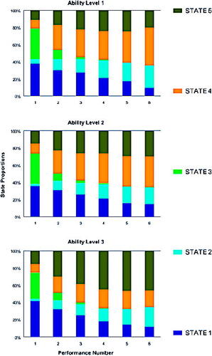
Figure 8. Learning Trajectories Across Classrooms. The proportion of HMM state usage for students from four molecular biology discussion sections are plotted for the six cases performed.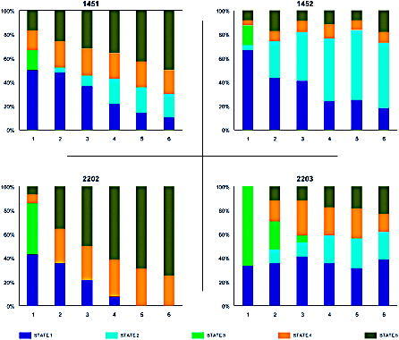
With experience, the student's knowledge base becomes qualitatively more structured and quantitatively deeper. This should be reflected in the way competent students or experts approach and solve difficult domain-related problems. In our model, State 4 would best represent the beginning of this stage of understanding. State 4 is a general all-purpose strategy by which most of the maps and laboratory data are ordered. It provides opportunities for both proving and eliminating hypotheses, and although not the most efficient approach, it has a reasonable success rate (78% for cases 1 and 3-6). On the most difficult case of the problem set, case 2, the solution frequency was only 55%, suggesting it is not a robust strategy for the more difficult problems.
Once experience was developed, students employed more effective and efficient strategies. This was most clearly shown by State 5 for which the solved rate was high and nodal analysis suggested selective test selections; State 2 would seem to be an even leaner strategy subset, and again, one not as robust as State 5 with the more difficult case 2 (68% solve rate vs. 77% solve rate). Not surprisingly, higher-achieving students had a higher proportion of performances in these states. What was interesting, and consistent with our previous observations, was that students appeared to stabilize their strategies by the fourth case performance, even though their solution frequency also stabilized at only 79%. Thus, one-fifth of the students may be comfortable with an approach that is neither efficient nor effective, and without an external intervention they could be at risk of failing to improve. Preliminary studies from a chemistry problem set under analysis suggests that learning in a collaborative group may be effective for jogging these students out of this state (Stevens et al., in press).
These studies also suggest that there were significant strategic differences across classrooms as evidenced by significant differences in the state learning trajectories across classroom settings. These were observed in the framing, transition, as well as the stabilization stages. These differences were not easily explained by differences in student abilities in the different sections. Because the sections were conducted on Monday, Tuesday, Wednesday, and Friday, one explanation was that students later in the week benefited from the experiences of the earlier students. A closer examination of the data suggested this may not be occurring, and in fact, going first may be an asset for strategic development. First, the overall solution frequency across the M, T, W, F sections was not significantly different (Pearson χ2 = 4.5, p = .209). Second, although the state distributions across the daily sections were significantly different (Pearson χ2 = 77.0, p < .000), the Monday periods actually had the highest proportions of State 5 performances, whereas the other sections had higher proportions of States 1 and 4 performances. In fact, detailed learning trajectory analysis showed that many of the students in the Monday sections followed the State 3. State 1. State 5 transition sequence, whereas the other sections more rapidly stabilized on State 4 strategies.
What specific suggestions can be extrapolated from these studies and models regarding the use of The lac Operon problem set in undergraduate classes? The first would be directed toward problem set development. The solution frequency for Case 2, one mutation dealing with regulation, was the lowest, suggesting that this was a topic in which the students could use more experience. From a data analysis perspective, having additional problem sets that vary in difficulty would also improve the modeling of student abilities by item response theory, as well as test the efficacy of our interventions. The dynamics of the learning trajectory models would also suggest that when the state information was reported back to faculty in an easy-to-understand form, then by the third or fourth performance, instructors in the discussion sections could begin to engage in interventions to improve the development of student strategies. These interventions could be targeted either to individual students in classrooms where most students are making good progress, or performed in group sessions in which an entire section is struggling with the concepts. One of the benefits of this form of modeling, however, is that it may be able to determine rapidly the effectiveness of the interventions.
From previous studies, when given enough data about a student's previous performances, hidden Markov model models have performed at more than 90% accuracy when tasked to predict the most likely problem solving strategy the student will apply next. This, in part, results from the stabilization of strategic approaches by students. Knowing whether a student is likely to continue to use an inefficient problem-solving strategy allows us to help the student in a timely way. Perhaps more interesting is the possibility that knowing the distribution of students' problem-solving strategies and their most likely future behaviors may allow us to construct strategic collaborative learning groups that optimize interstudent learning and minimize teacher interventions.
One of the greatest benefits of predicting future performances, however, will be the ability to form experimental groups and to test potential educational interventions by observing which interventions cause which students to deviate from inefficient learning trajectories.
APPENDICES A-C
Appendices A, B, and C summarize the data flow for three students. At the top of each figure is a written summary of the student of how he or she approached the problem set. The first column summarizes the performance data of the student on each of the cases (that were randomly delivered). Next, there is a search path map visualizing the steps performed on each of the cases; refer to Figure 2 for an expanded template map. The fourth column shows the neural network nodal classification of the performance indicating the node number and the number of total performances (of 3,599) that were clustered at that node. Finally, the last column relates the performance to the state derived from the hidden Markov modeling.


FOOTNOTES
Monitoring Editor: Deborah Allen DOI: 10.1187/cbe.04-03-0036
§ Present address: Institute for Defense Analyses, Science and Technology Division, 4850 Mark Center Drive, Alexandria, VA 22311.
ACKNOWLEDGMENTS
Supported in part by grants from the National Science Foundation (NSF-ROLE 0231995, DUE Award 0126050, ESE 9453918), the PT3 Program of the U.S. Department of Education (Implementation Grant, P342A-990532), and the Howard Hughes Medical Institute Precollege Initiative.


